Study of static and cyclic strains using the metal magnetic memory method

Corresponding Member of the Russian Academy of Sciences N.A. Makhutov (RAS Institute of Engineering Science)
Dr. A.A. Dubov, A.S. Denisov (Energodiagnostika Co. Ltd.)

Some results of investigation of mechanical and physical properties of steel specimens using the metal magnetic memory method were presented in papers [1, 2].

The above-mentioned investigations were carried out basically under the conditions of static tensile loading. Paper [3] presents some fragments of investigations of steel specimens under the conditions of cyclic tensile loading using the metal magnetic memory (MMM) method.

The need to check experimentally the correlation of diagnostic parameters with strain prompted carrying out of static and cyclic load testing of steel specimens by the MMM method. The necessity of such testing using the MMM method is also conditioned by the existing drawbacks in practical realization of cyclic strength testing of specimens.

These include, first of all, the difficulty of ensuring the continuous recording of the strain diagram synchronously with the amplitude and frequency of the load during the entire period of the cyclic load application right up to failure of the specimen. For recording of strain cycling diagrams in the course of loading, as a rule, lower frequencies are selected in order to ensure the recording accuracy of load parameters.

Secondly, there are no available physical methods of experimental investigations, which would allow the real-time tracing, synchronously with the load frequency, of physical processes of resistance to strain, occurring in the metal of specimens, in the course of cyclic loading.

During the last years attempts have been made to use the Acoustic Emission (AE) method for this purpose. However impossibility to install the AE sensors directly in the area of the assumed failure of the specimen and presence of the extraneous noise generated by operation of the testing machine complicate the AE investigations during such tests.

The first attempts to use the MMM and the appropriate inspection instruments for this purpose, presented in paper [3], showed good results. The small-sized sensors of the instruments, used by the MMM method, allow to install them directly near the location of the assumed failure (with the accuracy of up to 1 mm). At the same time, in contrast to the AE sensors, the direct contact of the sensor with the surface of the specimen is not required. Besides, the use of two- and three-component sensors allows, due to the magnetomechanical effect, tracing the variation of the strain amplitude in three directions: in the longitudinal (coaxially with the direction of the internal load), transverse (perpendicular to the applied load) and radial direction. At the same time the specialized TSC (Tester of Stress Concentration) instruments, equipped with a screen and a memory unit of 32 MB and higher, when operated in the “timer” mode, ensure continuous observation of the cyclic loading process of the specimen as well as on-line recording of measurement results of magnetic parameters synchronously with the applied cyclic load in a wide range of frequencies variation (from 1 Hz to 300 Hz).

Fig.1 shows the scheme of measurement of the normal and the tangential (in the direction of the applied load P) components of the self-magnetic field of the specimen placed in the tensile-testing machine. The specimen 2, which has a special groove 3 for localization of the inspection area, was fixed in the attachment unit 1 of the tensile-testing machine using two bolted joints. The two-component sensor 4, allowing to measure the tangential H_x and the normal H_y components of the magnetic field near the surface of the specimen (at the distance of 0.5÷1.0 mm), is installed in the holder 6 and fixed in it rigidly in one position. The electronic unit 5 – the analog-digital transducer – was connected to the recording TSC instrument.

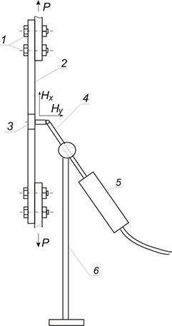
Let us further consider some results of steel specimens investigation during application of the cyclic tensile load in the range from 1 to 10 Hz. Testing of specimens according to the measurement scheme, presented in fig.1, was carried out at the A.A. Blagonravov Institute of Engineering Science of RAS using the testing machine “Material Test System (MTS) 311.21”.

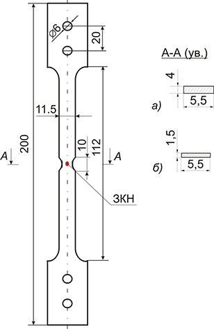
Fig.2 shows the shape and dimensions of the steel specimens used for cyclic tensile load tests. The cross-section restriction was made in the middle part of the specimens in order to determine the location of the assumed failure and of the maximum deformation of the specimen (SCZ) and, respectively, in order to determine the location of the TSC instrument sensor installation. The Ø 6 mm holes on the holders of the specimen were made to fit the bolted joints with holders of the testing machine. Two types of specimens were tested:

• type I, the material was the structural steel 10CrSND with the yield strength σ_y=450 MPa, ultimate strength σ_t=570 MPa and the area of the cross-section F=5.5×4=22 mm²;
• type II, the material was Steel 3 with the yield strength σ_y=250 MPa, ultimate strength σ_t=350 MPa and the area of the cross-section F=6.5×1.5=9.75 mm².

Four specimens of the type I and five specimens of the type II were tested in total. One specimen of each type was preliminarily subject to static tensile testing in order to determine the actual values of σ_y and σ_t. At the same time simultaneous recording (in the mode of the real-time application of the tensile load) of the strain diagram by the recording device of the testing machine and of variation of the normal (ΔH_y) and the tangential (ΔH_x) components of the magnetic field in the SCZ of the specimen was performed.

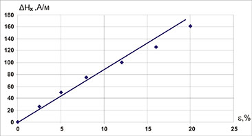
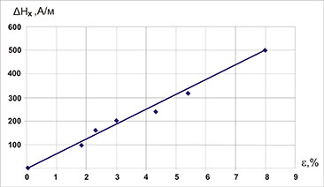
Fig.3 and fig.4 present comparison of the strain diagram σ-ε and the variation diagram of the tangential component of the magnetic field ΔH_x depending on tensile stresses, respectively, for the specimen of the type I and the specimen of the type II.

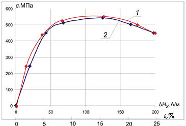
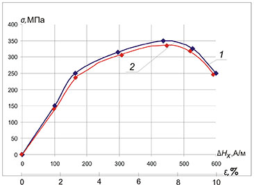
Fig.3 and fig.4 show good correlation between the obtained diagrams, which confirms the proportional dependence of variation of the self-magnetic field ΔH_x of the specimen on the tensile strain at the physical level.

Fig.5 and fig.6 show variations of the magnetic field ΔH_x depending on strain ε, obtained based on the results of measurements in SCZ (the neck zone), respectively, for the specimens of the type I and type II. It can be seen that the dependence ΔH_x=f(ε) has the linear and proportional nature.

Then three specimens (#2, #3, #4) of the type I and four specimens (#2, #3, #4, #5) of the type II were tested for cyclic tensile load at different frequencies.

Specimens of the type I were tested in the range of the tensile load from P_min=100 kg to P_max=950 kg or (0.2÷0.95)σ_y.

Specimens of the type II were tested in the range of the tensile load from P_min=50 kg to P_max=250 kg or (0.2÷1.0)σ_y.

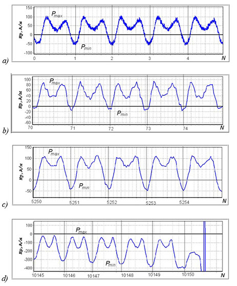
Fig.7 and fig.8 present time dependences of the normal H_y and the tangential H_x components of the magnetic field on the cyclic load, obtained during testing, respectively, for the specimen #3 of the type I (at the frequency of 2Hz) and for the specimen #4 of the type I (at the frequency of 10Hz).

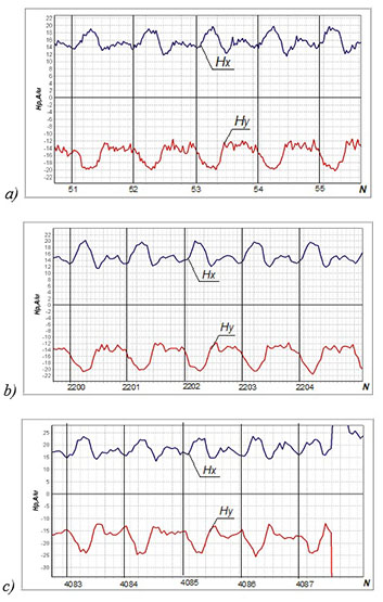
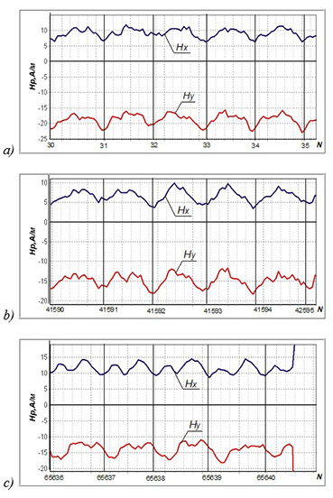
The general rules, which can be marked out based on the analysis of the magnetograms, presented in fig.7 and fig.8, are the following:

• coincidence by the frequency of the applied load and of the amplitude variation of the components H_y and H_x of the field;
• minor amplitude variation of the value of the field components H_y and H_x from the amplitude of the applied load at all stages of load cycles N right up to failure of the specimens;
• the number of cycles before failure of the specimen increases significantly with increasing of the frequency of the applied load from 2Hz to 10Hz.

Fig.9 shows the time dependence of the tangential H_x component of the magnetic field on the cyclic tensile load, obtained during testing of the specimen #2 of the type II at different stages of cyclic straining right up to failure. Based on the presented in fig.9 magnetograms, the following specific features can be pointed out:

• notable increasing of the amplitude variation of the H_x component of the field with increasing of the number of load cycles N (at the initial stage the modular variation is |ΔH_х|≈150 A/m, in the established mode |ΔH_х|≈200 A/m and at the final stage |ΔH_х|≈350 A/m);
• the effect of abrupt decline and instantaneous growth of the field H_x was recorded at the maximum of the applied load P_max of each cycle. The above-mentioned effect was not observed at the minimum of the cyclic load amplitude P_min. This effect was observed for both components of the field H_y and H_x, both for the specimens of the type II and for the specimens of the type I (see fig.7 and fig.8).

It should be noted that the display of the effect of short-time decline and growth of the field components H_y and H_x at the maximum of the cyclic tensile load increases gradually as the number of cycles grows and meets the maximum value by the amplitude directly before failure of the specimen. On both specimens of the type II (Steel 3) the variation amplitude of the field components H_y and H_x is notably greater as compared to the specimens of the type I (Steel 10CrSND).

Fig.10 presents the diagram of cyclic straining σ-ε, recorded on the specimen #2 of the type II for cyclic tensile loading in the range of (0.2÷1.0)σ_y. In this diagram the frequency of load application was reduced from 3 Hz to 1 Hz and lower. The comparison of fig.10 and fig.9 demonstrates that the diagram σ-ε does not observe the effect of short-time growth and decline of resistance to straining at the maximum of the applied load.

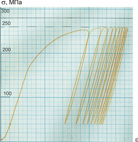
However the general pattern of the curve σ-ε (the width of the loop) at the load maximum corresponds to the magnetogram presented in fig.9. At the minimum of the cyclic load the appearance of the diagram σ-ε practically corresponds to the magnetogram presented in fig.9.

Fig.11 and fig.12 present variation of the tangential component of the magnetic field ΔH_x depending on the number of load cycles N, recorded during testing, respectively, of the specimen #4 of the type I and of the specimen #2 of the type II.

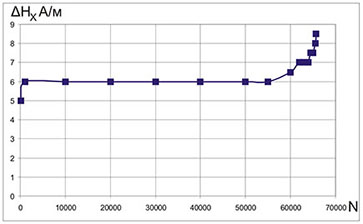
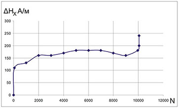
According to the rules established in the paper [4], the curves ΔH_x=f(N), presented in fig.11 and fig.12, qualitatively correspond to fatigue curves of the metal of the specimens.

These curves provide a unique opportunity to carry out the assessment of the process of fatigue time-dependent failure of the specimens depending on the number of cycles and the load frequency and amplitude. It should be noted that at present lifetime assessment of metal components using the diagnostic parameters of the MMM method (variation of the magnetic field ΔH and its gradient ΔH/Δx in SCZs) is applied successfully in practice.

Analysis of the results and conclusions

1. The obtained results of specimens investigation confirmed experimentally the earlier drawn conclusion about the possibility of application of the MMM method and of the appropriate inspection instruments for quick testing of mechanical properties and cyclic strength parameters at the physical level.

2. Comparison of strain diagrams σ-ε and magnetograms σ-ΔH_x, ΔH_x-ε, obtained in the mode of static loading (see fig.3, fig.4, fig.5, fig.6), of the diagrams of cyclic loading σ-ε (see fig.10) and corresponding magnetograms (see fig.7, 8, 9) confirms once more the earlier established correlation of magnetomechanical parameters, conditioned by the "magnetodislocation hysteresis".

3. In the process of cyclic loading a linear dependence was established between the amplitude of resistance to straining Δε and the variation amplitude of the self-magnetic field ΔH of the metal of the specimen.

4. The effect of abrupt decline and instantaneous growth of resistance to straining was recorded for the first time at the maximum of the applied tensile load of each cycle using the parameters of the magnetic memory of metal. The above-mentioned effect was not observed at the minimum of the amplitude of the cyclic tensile load. The display of the effect of short-time variation of resistance to straining at the maximum of the cyclic tensile load increases gradually as the number of cycles grows and meets the maximum value by the amplitude between the decline and growth of resistance to straining directly before failure of the specimen. Based on the earlier conducted experimental investigations [2] it can be assumed that the revealed effect characterizes growth of metal damaging in the form of accumulation and gradual increasing of dislocations density in a SCZ, being the site of potential failure of the specimen.

5. The fatigue curves, plotted by variation of the self-magnetic field of the specimens in the course of cyclic loading, confirm experimentally the possibility of lifetime assessment of metal components by the parameters of the magnetic memory of metal.

6. The magnetograms, recorded during cyclic loading of specimens in the real-time mode, allow declaring the possibility to use the MMM method and the TSC-type instruments for monitoring of the technical state directly during operation of the pressure equipment. Taking into account that various types of noise do not influence the diagnostic parameters of the MMM method and that no special additional loading is required, the TSC-type instruments and the appropriate sensors (which do not require the direct contact with the inspection object) have obvious advantage over the AE instruments, which are widely used in practice for monitoring of the technical state of metal components.

References

1. A.A. Dubov. Investigation of metal properties using the effect of the magnetic memory of metal // Physical metallurgy and heat treatment of metals, 1997, No.9.

2. V.M. Goritsky, A.A. Dubov, E.A. Demin. Investigation of structural damageability of steel samples using the metal magnetic memory method // Control. Diagnostics, 2000, No.7.

3. А.А. Dubov, Аl.А. Dubov, S.М. Kolokolnikov. The metal magnetic memory method and inspection instruments. Training handbook. Moscow: ZAO "Tisso", 2008. 365 p.

4. V.T. Vlasov, А.А. Dubov. Physical bases of the metal magnetic memory method. Moscow: ZAO "Tisso", 2004. 424 p.