On relationship of magnetic, acoustic and mechanical characteristics assessed during tensile testing of steel specimens

A.A. Dubov, N.A. Semashko, V.Yu. Privalov (Energodiagnostika Co. Ltd.)
L.R. Botvina, A.B. Tsepelev (IMET RAS)

Introduction

To assess the residual life of units and parts during operation, methods of stress state non-destructive testing are used, most of which allow to obtain only information on the average level of internal stresses that, as a rule, does not exceed the yield strength. At the same time, it is known that the material failure most often occurs in local stress concentration zones, where the processes of corrosion and fatigue damage develop intensively. The size of such zones varies from micrometers to units of millimeters, and the magnitude of internal stresses in them can significantly exceed not only the yield strength, but also the tensile strength of the material.

To detect stress concentration zones in loaded structures, it is promising to use the methods of metal magnetic memory (MMM) [1] and acoustic emission (AE) [2], but for the practical application of these methods, it is necessary to establish the relationship of magnetic and acoustic parameters with strength characteristics including proportional limits (σ_pr.lim.), yield (σ_0,2) and strength (σ_t).

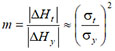
Previously, in papers [1, 3], when testing specimens of structural steels, the relationship was established between the ratio of magnetic field gradients (|ΔH|), measured at yield strength (|ΔH_y|) and the tensile strength (|ΔH_t|) with the ratio of the tensile strength to the yield strength:

Relation (1), reflecting this relationship, was called "energy" [3, 4], since the magnetic field gradient |ΔH| characterizes the density of magnetic energy W_m due to mechanical strain energy under loading W_с:

|ΔH| ~ W_m(W_c).

This paper describes the mechanical tests of structural carbon steel 20 under tensile conditions during the simultaneous monitoring of specimens' magnetic and acoustic properties using the MMM and AE methods. The work was aimed at determining the correlation relationships between MMM and AE parameters and strength characteristics (σ_t, σ_y) of steel.

Test procedure

The studies were carried out on structural carbon quality steel 20 (GOST 1050-88) specimens in the shape of a double blade with the working part cross section of 10 × 2,33 mm (Figure 1).

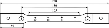
Tensile tests were performed on a 1958Y-10-1 tensile testing machine at the specimen movable clamp travel speed of 2.5 mm/min. The self-magnetic field of the specimen was measured in accordance with the procedure [1] using four three-component sensors mounted along the working part of the specimen in close proximity to its surface at an equal distance from each other (Figure 1). MMM sensors were connected to a TSC-5M-32 type magnetometer with a recording device and a memory unit. Based on the results obtained using the three-component sensors and the ratio

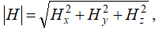
the resulting magnetic field intensity was calculated at each point of the specimen.

For acoustic pulses recording and processing, the СДС 1008 acoustic emission system was used, which includes a system unit and a personal computer with software ("Maestro" software). AE sensors were mounted between the testing machine clamps and the specimen working part at points 1 and 2 (Figure 1).

Results and discussion

Figure 2 shows a graph of the resulting magnetic field Н time variation at the point closest to the place of specimen rupture (А - the initial state of the specimen under load P=0).

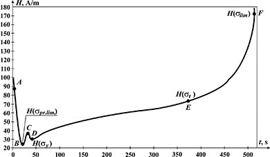
With load increase, the magnetic field H intensity decreases sharply (in section A–B, Figure 2), reaches two minimums at points B, D, and an intermediate maximum at point C. It was found that points B, D correspond to the proportional limit and the yield strength of the material, assessed by analyzing the strain curve. Point C corresponds to the yield drop on the strain curve for mild steel.

Further increase in the H field intensity in the D-E section occurs in the area of the specimen uniform strain up to reaching the tensile strength σ_t. After this, rapid (power-law) growth of H values in the Е-F region is observed right up to the specimen ruptures. Point F in Figure 2 corresponds to the true limit stress value σ_lim, which can be assessed taking into account the specimen's cross-sectional area reduction before failure.

Papers [3–5] demonstrated the possibility to determine the location of strain and, accordingly, the place of the future neck formation by the maximum variation (in absolute value) of the magnetic field intensity |ΔH| in section AB. In our case, the maximum variation |ΔH| in section AB was recorded by sensor III (Figure 1), which, as it turned out later, was located near the place of the specimen rupture. Comparison of the measured dependence H(t) with the load curve σ(ε) prompts that the value σ_pr.lim. for this specimen is ~ 0,4σ_t.

Based on the data shown in Figure 2, the graph of cumulative modular values of the resulting field intensity variation due to strain was plotted (here |ΔH_i| – field variation in the selected (A–B, B–C, and C–D) and subsequent sections of the H(t) curve with duration of 50 seconds, n – the number of sections). The graph plotted in this way and presented in Figure 3 along with the strain curve for the same specimen, made it possible to assess the modular values of the total magnetic field intensity variation ∑|ΔH_y|, ∑|ΔH_t| and ∑|ΔH_lim|, corresponding to the characteristic points on the strain curve: yield strength, tensile strength and the limiting stress value in the specimen neck at the time of its failure.

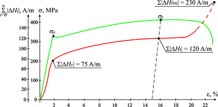
Based on the obtained data, a "magnetic indicator" m was estimated [1]:

The value of this indicator turned out to be close to squared ratio of the tensile strength and yield strength:

Thus, m values, obtained from the magnetic and mechanical characteristics, practically coincide. This means that by using the results of standard tensile tests of specimens and the relation (1), it is possible to determine the limiting value of the parameter m for real engineering structures made of the same material.

Let us now consider the acoustic emission signal readings obtained during the specimen tensile testing. Figure 4 shows the time dependences of the count rate (1) and the total AE pulse count (∑N) (2). Curve 2 shows the points corresponding to the material's yield strength σ_y and tensile strength σ_t estimated based on the tensile diagram.

From Figure 4 it follows that the total count value ∑N at the yield strength is ~ 175 pulses, and at the tensile strength ~ 275 pulses, and their ratio is: 275/175=1.57, which is very close to the value of m obtained from the relationship (σ_t/σ_y)².

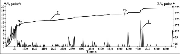
Figure 5 shows the time dependence of AE signal energy parameters during the tensile testing. Signals 1 in Figure 5 reflect the energy of single signals over time (E), and curve 2 displays the total AE energy (∑Е) during the specimen tensile testing time. Curve 2 shows the points corresponding to the specimen's yield strength σ_y and tensile strength σ_t.

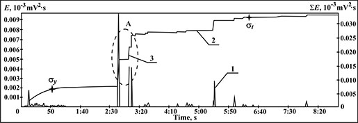
The value of AE pulse total energy at the time when the tensile strength σ_t is reached is ∑Е_t=0.032 and the average value ∑Е^ave_A in the curve 2 section from the yield strength σ_y to zone A (maximum energy release) is 0.020 (see Figure 5). Thus, the ratio ∑Е_t / ∑E^ave_A =0.032/0.020=1.6, which is also close to the values of m obtained from relation (1) based on the magnetic measurements and mechanical test data.

Since the magnetic field values in the area of maximum strain localization close to the specimen rupture point was used to determine the value of the magnetic indicator m using the relation (1), the MMM and AE parameters were compared based on measurements in the "neck" zone of the specimen.

Analysis of the acoustic pulse radiation location map in the course of the specimen strain showed that zone A in Figure 5, recorded by AE signal sources in ∑Е curve section between σ_y and σ_t, coincides with the site of strain localization and subsequent specimen rupture. The fact that the position of one of the magnetic sensors coincides with strain localization site provided good consistency of the numerical data obtained from relation (1) with the results of MMM and AE parameters measuring during the tensile testing of the same specimen.

The studies were carried out with financial support from the Russian Science Foundation grant (project No. 15-19-00237).

Conclusions

1. The values of the self-magnetic field intensity variation and acoustic emission parameters were estimated in the course of a mild steel specimen tensile testing.

2. It was shown that the ratio of magnetic field intensity modular values in the strain localization zone, corresponding to the tensile strength and yield strength, is close to squared ratio of these very characteristics (tensile strength to yield strength).

3. Application of the magnetic memory method makes it possible to estimate the true limiting failure stress.

4. The values of the ratio of AE pulse total energy before the tensile strength in the strain localization zone to the average value of this characteristic are estimated. It was shown that this ratio is also close to squared ratio of the tensile strength and the yield strength.

5. The established relationship of physical characteristics variation with mechanical properties can form the basis for quantitative assessment of material damage and residual life of real structures during their operation.

References

1. A.A. Dubov, Al.A. Dubov, S.M. Kolokolnikov. Metal magnetic memory method and inspection instruments: Training Handbook – Fifth edition. Moscow: Publishing House "Spektr", 2012. 395 p.

2. N.A. Semashko, V.M. Shport. Acoustic emission in experimental engineering. Moscow: Mashinostroyenie, 2002. 320 p.

3. V.T. Vlasov, A.A. Dubov. Physical theory of the "strain-failure" process. Part I. Physical criteria of metal's limiting states. Moscow: Publishing House "Spektr", 2013. 488 p.

4. N.A. Makhutov, A.A. Dubov, A.S. Denisov. Study of static and cyclic strains using the metal magnetic memory method // Zavodskaya laboratoriya, 2008, No.3. pp. 42-46.

5. V.T. Vlasov, A.A. Dubov. Physical bases of the metal magnetic memory method. Moscow: ZAO "Tisso", 2004, 424 p.